Functional Random Forest (FRF) Manual
The Functional Random Forest presented in Subtyping cognitive profiles in Autism Spectrum Disorder using a random forest algorithm, E. Feczko Ph.D. et al.
This manual documents how to use the RFAnalysis package written by Eric Feczko. The manual is split into two main sections. The first section covers how to analyze cross-sectional data with the Random forest subgroup detection (RFSD) tool. The second covers how to analyze longitudinal trajectories with the Function Random Forest (FRF) tool. A brief introduction will walk the user through installing the software.
Installation
Getting the package
The FRF code can be found on the github repository. This repository is intended for public release as a stable build. For the developmental builds please contact Eric Feczko (feczko@ohsu.edu) or the Fair Lab. The repository itself can be installed at any location through use of git:
git clone https://gitlab.com/feczko/Analysis /destination/path/for/FRF
Dependencies
There are two versions of the FRF, the source version and the compiled version. The source FRF has two external dependencies:
- MATLAB version 2016 or higher
- MATLAB Machine learning and statistical toolbox
- MATLAB Parallell Computing Toolbox [OPTIONAL]
The compiled FRF has one external dependency:
- The MATLAB compiler engine which should be provided by the Fair Lab.
Both the source and compiled versions also require that Infomap (http://mapequation.org) is installed on your system.
There is also a python2.7 dependency in this project, to support a simpler
interface to Infomap. In order to install this dependency you must install
python2.7numpyscipy
These can be installed to your system, or by use of virtualenv. The
instructions for this will are located here
Using the package in the matlab environment
FRF was designed such that an individual does not need to access the matlab IDE to run the data. If one is planning to use any of the matlab functions themselves, one will need to add the package to the MATLAB path. After starting matlab type:
addpath(genpath('/destination/path/for/Repository/'))
and the matlab functions will be available within a matlab session.
Random forest subgroup detection (RFSD)
Preparing your data
Generating your data file
The FRF package requires input data represented as a 2D numeric or 2D cell matrix stored in a .mat format. Each row contains an independent case and each column contains a feature (e.g. a predictor variable or the outcome measure). Usually, the source of the input data is external to matlab and will need to be represented as a variable and stored in the .mat format. Depending on the type of source, different steps can be taken to prepare the data properly.
NOTE that empty cells in your data set are expected to
be represented by NaNs before being passed into the RFSD algorithm.
If you have empty cells, or cells with only whitespace, in an excel spreadsheet,
the provided function PrepExcelSheetForTreeBagging will create a matlab struct
with correctly formatted data.
Excel
For excel spreadsheets, a function, PrepExcelSheetForTreeBagging can be used. In a MATLAB environment, add the package to your MATLAB path (see: “Using the package in the matlab environment” under “Installation”) type:
help PrepExcelSheetForTreeBagging
for documentation on usage.
On a command line, the PrepExcelSheetForTreeBagging_wrapper.sh can be
used to prepare your data from an excel sheet. The wrapper requires you
to create a parameter file, which can be modified from the existing
PrepExcelSheetForTreeBagging_example.bash file. The contents of the
file are reprinted below. Each parameter precedes its definition; all
definitions are noted by hashmarks, excluding the first line:
#!/bin/bash

# path and filename where the excel spreadsheet is located
excelfile=/path/to/excelfile/.xls

# the name of the output (.mat) file.
output_matfile=/path/to/dataset.mat

# if set to anything but 0 or blank, the first row of the excel file is
#   a header and will be ignored
exists_header=0

# a numeric vector encapsulated by square brackets, where each number
#   denotes a column that represents a categorical variable, set to 0 if
#   no such variable exists
string_cols=[2 3 4]

# sets whether the output contains rows with missing data ('surrogate')
#   or excludes the rows ('no_surrogate')
type='surrogate'

# the name of the variable saved to the .mat file
varname=group_data

# the full path to the repository containing the RFAnalysis code.
repopath=/destination/path/for/FRF

# the name of the matlab command line executable, can include arguments
#   additional options, etc. SingleCompThread is enabled by default.
matlab_command=matlab
After generating a parameter file, one can prepare their data using the wrapper. From a bash terminal, one can execute the wrapper on his or her parameter file:
./RFSD/PrepExcelSheetForTreeBagging_wrapper.sh parameterfile.bash
NOTE that parameter files in the RFSD directory end with the file
extension .bash. This is to help discern if a file is intended to be
an executable (ending in .sh) or a parameters file.
The output from PrepExcelSheetForTreebagging will be a .mat file containing your named variable. Both the variable name and path must be modified in the ConstructModelTreeBag wrapper below (see: “Running the analysis”).
R
If your data exists within an R data frame, R packages can be used to export the data frame as a .mat file explicitly (e.g. R.matlab: https://cran.r-project.org/web/packages/R.matlab/index.html). Since FRF accepts cell or numeric matrices, one can export a data frame as a cell matrix:
writeMat(con="…filepath",x=data)
or as a numeric matrix:
writeMat(con="…filepath",x=as.matrix(data))
R.matlab also enables one to load outputs into R for inspection (see: “loading outputs in R” under “Interpreting the Outputs”).
python
If your data is extracted using python, scipy can be used to export the
data as a .mat file explicitly. The data must be stored as a
NxM numpy array or list where rows represent the cases (N) and columns
represents the features.
data_mat=[]
data_mat.append(data)
scipy.io.savemat('group_data.mat', {'group_data':data_mat})
Scipy also enables one to load outputs into python for inspection (see: “loading outputs in python” under “Interpreting the Outputs”)
CSV
CSVs (comma separated value files) can be implicitly handled by the FRF package. To use a CSV as an input, the following steps have to be taken:
- The CSV must be organized as a table (i.e. 2D matrix) with rows representing cases and columns representing features.
- The delimiter used by the CSV
- The CSV cannot contain any header information (i.e. a top row depicting the column headers).
- Missing or blank cells (see: “How to deal with missing data”) must be represented by NaNs.
How to deal with missing data
Our RF approach can handle missing data via use of “surrogate splits”. Specifically, when the RF model encounters missing data in the training data set, it will generate a small RF from the bootstrapped training data only that attempts to fill that missing value. For sets of cases/variables where data is missing, the actions taken depends on whether the variable is categorical or continuous. For continuous variables, one should either the leave the cell blank (unless using CSVs) or replace all missing values with the value NaN (not a number). In the case where the variable is categorical, the variable must be left blank.
Surrogate splits are not a panacea. For example, consider the extreme situation where 95 percent of cases are missing the given feature. Even if one could successfully predict the feature value for the 95 percent of cases using other data, such a relationship would imply that the feature is derived from other features. Therefore, such a feature would not contribute anything unique to the model. In our experience, it is critical for the user to perform exploratory data analysis (EDA) on their own datasets. If more than 15 percent of a given case or a given variable is missing data, one should remove the given case or variable. One can toggle whether surrogate splits are used in the approach by modifying the parameter file (see: “Generating your parameter file”).
Generating your parameter file
The RFSD and FRF packages contain bash wrappers for executing the algorithm
from the command line. Parameter files are used to store the
configuration for the analysis. Below are the parameters available for
running the RFSD using the ConstructModelTreeBag_wrapper.sh. These
parameters can be found in the TreeBagParamFile_example.bash. We use this
configuration file in order to support the many user tuned parameters.
In order to understand the layout of this Parameters File, we provide some
intuition. Comments precede parameter definitions for clarity. Variable assigment
(in bash), requires no space around the = character.
File sections that follow the pattern below, describe a conditional relationshi
This relationship dictates that under a condition of variable_name,
subvariable_name_one and subvariable_name_two will be used and must be
defined. Otherwise, then these values will be ignored.
variable_name=false
    subvariable_name_one=monkey
    subvariable_name_two=7
Additionally, the use of 0 as an index denotes a false state. These tools
are written in matlab, and therefore assumes a 1 index of colunmns and arrays
Comments of the form below, are used to designate categories of defined variable
# =====================
# == Sectional Title
# =====================
Our example config file is found here.
Running the analysis
RFSD allows for multiple different workflows to analyze your data. The manual will cover two standard and two optional workflows:
- RFSD analysis
- RFSD power analysis
- [OPTIONAL] Rerun subgroup analysis
- [OPTIONAL] Perform community detection on a proximity matrix
RFSD analysis
Once you have prepared the parameter file, you can run the RFSD analysis using the ConstructModelTreeBag_wrapper.sh command.
./RFSD/ConstructModelTreeBag_wrapper.sh paramfile.bash
The runtime for ConstructModelTreeBag varies by multiple factors. Individual forests are affected by the complexity of the data, the number of trees, and model construction parameters like the number of variables examined per branch. Total runtime is affected by factors like the number of participants, and the type of validation performed. With OOB turned on each RF model increases in runtime as the number of subjects increases. With variable importance turned on, the runtime will increase by the number of variables.
Currently, we have not performed a rigorous analysis of how each factor affects runtime. For a 10-fold cross-validation with 3 repetitions on 1000 trees, the RF validation should take no more than an hour to complete, if out of bag (OOB) error and variable importance are turned off. It is recommended to perform a single large model (10 times as many trees) on one repetition when evaluating OOB error or variable importance; a single RF model may take 1-4 hours if these options are enabled.
Subgroup detection runtime depends on the type of classifer, and the number of edge densities explored, as set by the parameter file. With the defaults enabled, subgroup detection will take 4 hours on unsupervised or regression models, and up to 12 hours on supervised classifiation models.
RFSD power analysis
The RFSD power analysis can be used to estimate statistical power for unsupervised and supervised analyses. A parameter for the expected effect size (as measured by accuracy, mean absolute error, or subgroup similarity) must be selected by the user to calculate statistical power. A range of parameters can be selected if the expected effect size is unknown. A sample size must also be selected by the user. To run multiple sample sizes, one will need to generate parameter files for each sample size.
RFSD power analysis requires preparation of the RFSD parameter file. Because the power analysis is computationally intensive, we recommended using a computing cluster to enable parallelization of the simulations. The parameter file uses the same formatting as for the RFSD analysis, and can be found here.
Once you have prepared the parameter file, you can run the RFSD analysis using the RunRFSDPowerAnalysis_wrapper.sh command.
./RFSD/RunRFSDPowerAnalysis_wrapper.sh RFSD_paramfile.bash
Interpreting the outputs
Outputs are stored as .mat files, which encapsulate several matlab variables.
Although there are multiple intermediate outputs, only two contain the final
outputs from the analysis:
ExcelOutput.mat– as generated byPrepExcelSheetForTreeBagging.mand named by parameteroutput_matfile,filename.mat– as generated byConstructModelTreeBag.mand named by parameterfilename, contains relevant outputs from the RF modelsfilename_output/subgroup_community_assignments.mat– as generated byRunAndVisualizeCommunityDetection.mand named by parameterfilename, contains relevant outputs from the subgroup detectionRFSD_filename_output.mat– as generated byRunRFSDPowerAnalysis.mand named by parameteroutput_directory, contains outputs from the RFSD power analysis, such as statistical power and false positive rates.- If a supervised classifier is selected, additional intermediate outputs will
be saved in:
filename_output_groupX/– as generated byVisualizeTreeBaggingResults.mand named by parameterfilename, contains relevant outputs from group (class) number X
Stored outputs
Data dictionaries for output files are specified below.
ExcelOutput.mat data dictionary
| variable name | output from | used in | matlab datatype | R datatype | python datatype | dimensions | null value | description |
|---|---|---|---|---|---|---|---|---|
| group_data | PrepExcelSheetForTreeBagging | ConstructModelTreeBag, VisualizeTreeBaggingResults , RunRFSDPowerAnalysis | numeric matrix | data matrix | numpy array | 2 | cannot be null | Matlab formated matrix representing input data |
filename.mat data dictionary
| variable name | output from | used in | matlab datatype | R datatype | python datatype | dimensions | minimum value | maximum value | null value | description |
|---|---|---|---|---|---|---|---|---|---|---|
| accuracy | ConstructModelTreebag | VisualizeTreeBaggingResults | numeric matrix | data matrix | numpy array | 2-3 | -1 | 1 | cannot be null | model performance: first dimension reflects statistic type (e.g. group accuracy, total performance, error, or correlation), second dimension reflects repetition/fold index, third dimension reflects repetition index (if CV is enabled). |
| features | ConstructModelTreebag | VisualizeTreeBaggingResults | numeric matrix | data matrix | numpy array | 1 | 0 | +inf | cannot be null | #times each predictor is used |
| final_data | ConstructModelTreebag | VisualizeTreeBaggingResults | numeric matrix | data matrix | numpy array | 2 | depends on dataset | depends on dataset | cannot be null | data excluding the outcome variable, can be used with “subgroup_community_assignments” to evaluate features used |
| final_outcomes | ConstructModelTreebag | VisualizeTreeBaggingResults | numeric matrix | data matrix | numpy array | 1 | depends on dataset | depends on dataset | cannot be null | outcome_variable, can be used with “subgroup_community_assignments” to evaluate outcomes by subgroup |
| features | ConstructModelTreebag | VisualizeTreeBaggingResults | numeric matrix | data matrix | numpy array | 1 | 0 | +inf | cannot be null | #times each predictor is used |
| group1class | ConstructModelTreebag | VisualizeTreeBaggingResults | numeric matrix | data matrix | numpy array | 1 | -1 | 1 | cannot be null | individual performance for first dataset |
| group1predict | ConstructModelTreebag | VisualizeTreeBaggingResults | numeric matrix | data matrix | numpy array | 1 | outcome dependent | outcome dependent | cannot be null | model prediction for first dataset |
| group1scores | ConstructModelTreebag | VisualizeTreeBaggingResults | numeric matrix | data matrix | numpy array | 1 | outcome dependent | outcome dependent | cannot be null | model score for first dataset |
| group2class | ConstructModelTreebag | VisualizeTreeBaggingResults | numeric matrix | data matrix | numpy array | 1 | -1 | 1 | NaN | individual performance for second dataset |
| group2predict | ConstructModelTreebag | VisualizeTreeBaggingResults | numeric matrix | data matrix | numpy array | 1 | outcome dependent | outcome dependent | NaN | model prediction for second dataset |
| group2scores | ConstructModelTreebag | VisualizeTreeBaggingResults | numeric matrix | data matrix | numpy array | 1 | outcome dependent | outcome dependent | NaN | model score for second dataset |
| npredictors | ConstructModelTreebag | VisualizeTreeBaggingResults | numeric | int32 | int32 | scalar | 1 | # of features | NaN | number of predictors used to grow each branch |
| outofbag_error | ConstructModelTreebag | VisualizeTreeBaggingResults | numeric matrix | data matrix | numpy array | 2 | 0 | 1 | NaN | Cumulative OOB error: first dimension reflects repetition index, second dimension reflects # of trees |
| outofbag_varimp | ConstructModelTreebag | VisualizeTreeBaggingResults | numeric matrix | data matrix | numpy array | 2 | -1 | 1 | NaN | OOB measured variable importance: first dimension reflects repetition index, second dimension reflects feature index |
| permute_accuracy | ConstructModelTreebag | VisualizeTreeBaggingResults | numeric matrix | data matrix | numpy array | 2-3 | -1 | 1 | NaN | Null model performance. See “accuracy” for format. |
| proxmat | ConstructModelTreebag | RunAndVisualizeCommunityDetection | cell matrix | list of data matrices | list of numpy arrays | 1 | 0 | 1 | cannot be null | NxN proximity matrices generated from the RF, one per forest is saved to limit space. N refers to the number of subjects. If group2_validate_only is set to true, then the proximity matrix will only reflect the independent testing dataset. |
| treebag | ConstructModelTreebag | ConstructModelTreeBag | cell matrix containing RF objects | N/A | N/A | 1 | N/A | N/A | NaN | this variable contains each model generated from the RF validation. The size of the matrix depends on the number of forests generated. Each model is stored as a TreeBagger class object, and cannot be loaded yet in R or python. |
| trimmed_features | ConstructModelTreebag | R/MATLAB/python | data matrix | numpy array | 2-3 | 1 | # of features | NaN | NaN | If features were trimmed using the legacy “estimate_features” option, this variable contains an index of which features were used. We do not advise using this feature. |
filename_output/subgroup_community_assignments.mat data dictionary
| variable name | output from | used in | matlab datatype | R datatype | python datatype | dimensions | minimum value | maximum value | null value | description |
|---|---|---|---|---|---|---|---|---|---|---|
| community_subgroup_performance | VisualizeTreeBaggingResults | R/MATLAB/python | cell matrix | list of lists | list of numpy arrays | 1 | -1 | 1 | cannot be null | Contains the model performance for each individual, split first by class, then by subgroup within class. Each subgroup list contains a matrix of number reflecting performance. Mean absolute error is used for regression, accuracy for classification. |
| subgroup_community_assignments | VisualizeTreeBaggingResults | R/MATLAB/python | cell matrix | list | list | 1 | G1_1 | GX_Xs | cannot be null | list of subgroups identified by the RFSD, X refers to the class, Xs refers to the subgroup within the class |
| subgroup_community_num | VisualizeTreeBaggingResults | R/MATLAB/python | numeric matrix | data matrix | numpy array | 2 | 1 | +inf | cannot be null | numeric representation of subgroup_community_assignments: first column represents the class index, second column represents the subgroup index for that subject |
| subgroup_communities | VisualizeTreeBaggingResults | R/MATLAB/python | cell matrix | list of data matrices | list of numpy arrays | 1 | 1 | +inf | cannot be null | list of subgroup communities for each class |
| subgroup_sorting_orders | VisualizeTreeBaggingResults | R/MATLAB/python | cell matrix | list of data matrices | list of numpy arrays | 1 | 1 | # of cases | cannot be null | list of order of subjects in the other variables split by subgroup, can be used to query “filename_output.mat” |
| proxmat_subgroup_sorted | VisualizeTreeBaggingResults | R/MATLAB/python | numeric_matrix | data matrix | numpy array | 2 | 0 | 1 | cannot be null | The mean proximity matrix (NxN where N is the number of cases) sorted first by class and then by subgroup. |
RFSD_filename_output.mat data dictionary
| variable name | output from | used in | matlab datatype | R datatype | python datatype | dimensions | minimum value | maximum value | null value | description |
|---|---|---|---|---|---|---|---|---|---|---|
| observed_performance | RunRFSDPowerAnalysis | R/MATLAB/python | numeric matrix | data matrix | numpy array | 2 | -1 | 1 | cannot be null | performance when H=1, depending on the question, multiple performances may be observed, rows contain different metrics, columns contain different runs |
| null_performance | RunRFSDPowerAnalysis | R/MATLAB/python | numeric matrix | data matrix | numpy array | 2 | -1 | 1 | cannot be null | performance when H=0, depending on the question, multiple performance metrics may be calculated, rows contain different metrics, columns contain different runs |
| sample_size | RunRFSDPowerAnalysis | R/MATLAB/python | numeric | int32 | int32 | 1 | 1 | +inf | cannot be null | sample size specified by the user in the parameter file |
| statistical_power | RunRFSDPowerAnalysis | R/MATLAB/python | numeric matrix | data matrix | numpy array | 2 | 0 | 1 | cannot be null | statistical power for each performance metric. Rows contain different performance metrics, columns contain different runs. First row represents the study power. |
| false_positive | RunRFSDPowerAnalysis | R/MATLAB/python | numeric matrix | data matrix | numpy array | 2 | 0 | 1 | cannot be null | false positive rate for each performance metric. Rows contain different performance metrics, columns contain different runs. First row represents the study power. |
| performance_thresholds | RunRFSDPowerAnalysis | R/MATLAB/python | numeric_matrix | data matrix | numpy array | 1 | 0 | 1 | cannot be null | performance threshold(s) specified by the user |
Data dictionaries will be expanded for non-critical outputs in upcoming releases. Please contact the development team via github for questions and requests.
Loading outputs externally
All output matlab files are stored in HDF5 format. Therefore,
any software package that can read HDF5. Below are HDF5 packages that should
work with our formats.
- R: “http://bioconductor.org/biocLite.R”
- Python: “https://www.h5py.org/”
The other packages below should also be able to load the outputs.
Loading outputs in R
Output matlab files can be read into R using the R.matlab package.
FRF_outputs <- readmat(con="filename.mat")
Outputs are represented as integers, data matrices and lists. Please consult the respective data dictionary for variable names and formatting. Data visualization R scripts are available and will be documented in a future release.
Loading outputs in python
Output matlab files can be read into python using scipy.
FRF_outputs = scipy.io.loadmat('filename.mat')
Outputs are represented as numpy arrays, integers, and lists. Please consult the respective data dictionary for variable names and formatting. Python data visualization code is planned for a future release.
Data visualizations
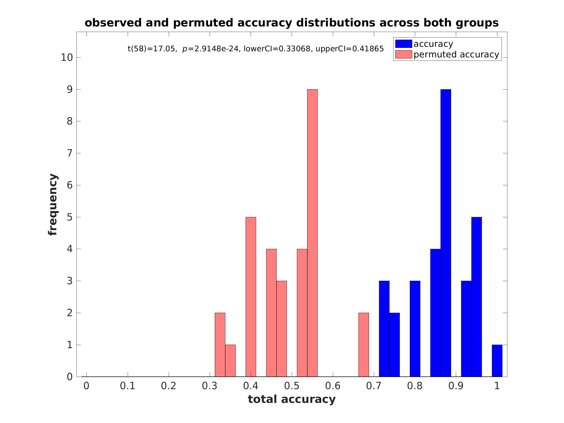
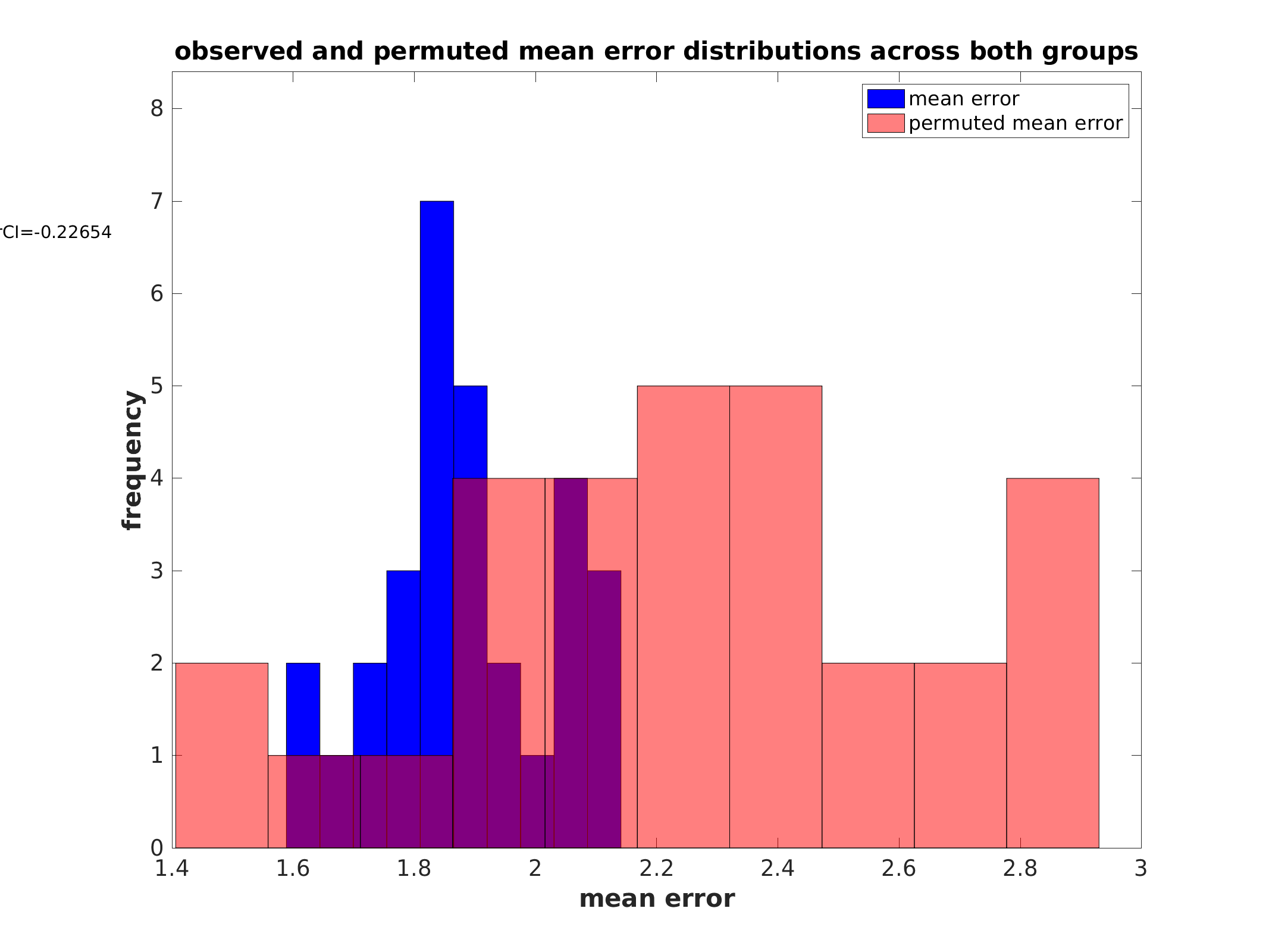
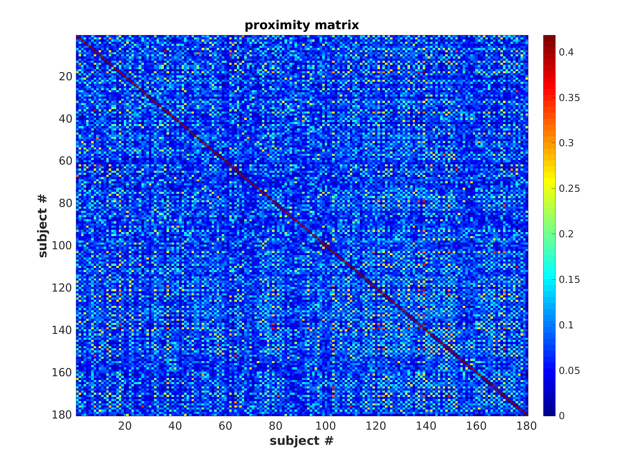
Examples of data visualizations are shown below. Examples will be added with new releases.
Performance histograms (classification):
Performance histograms (regression):
Proximity matrix (unsorted)
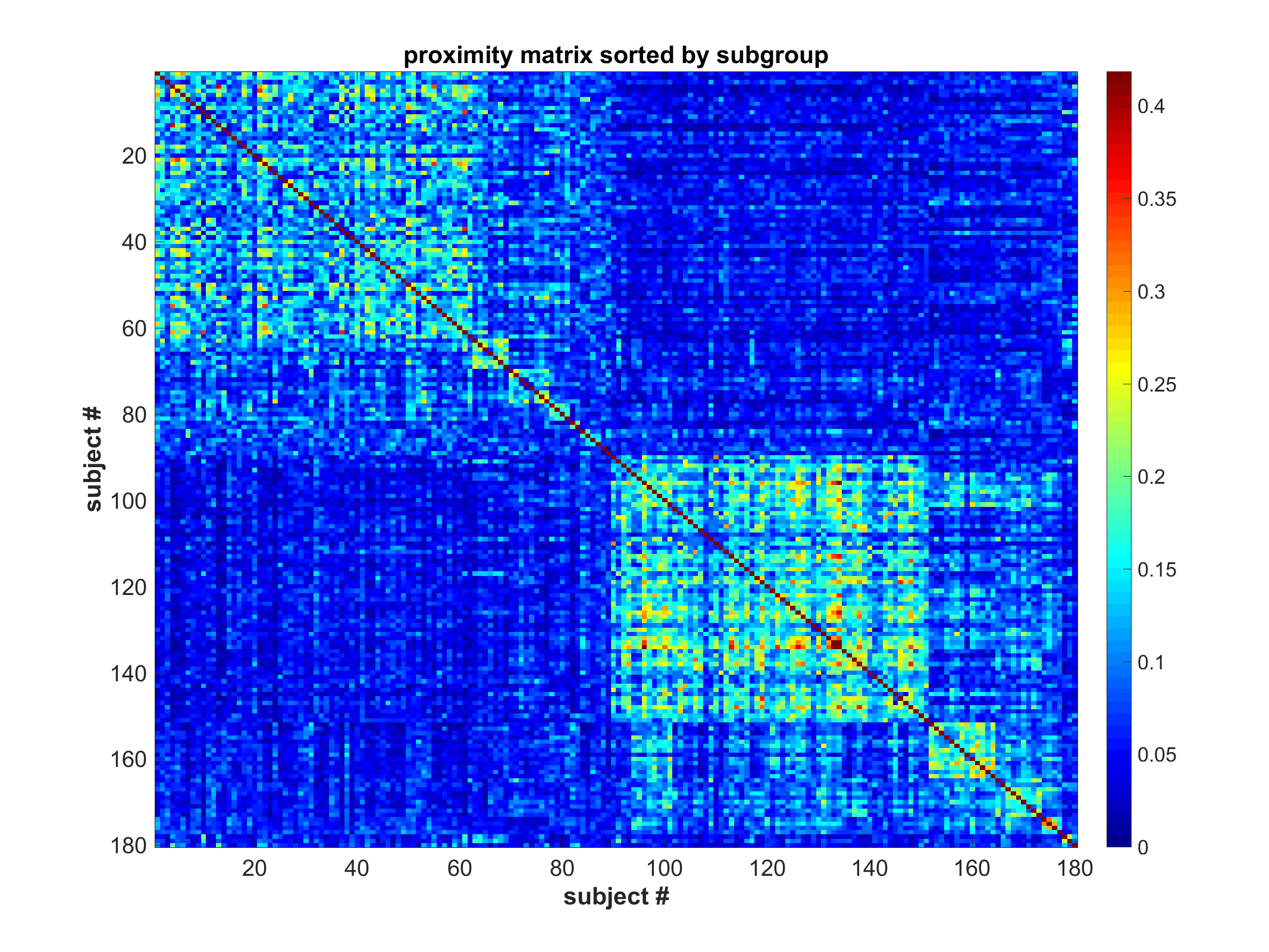
Proximity matrix (sorted)
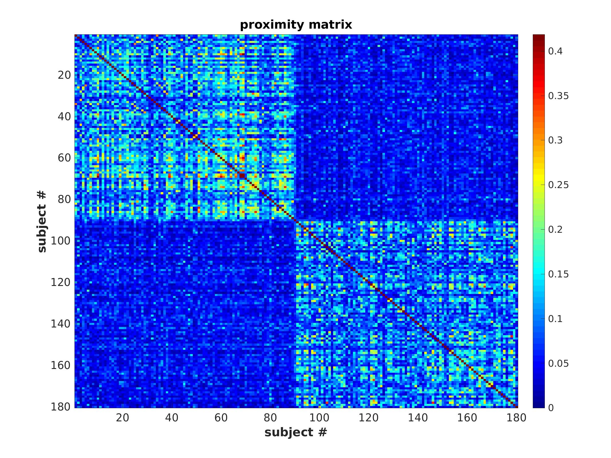
Proximity matrix sorted by subgroup and class (if available)
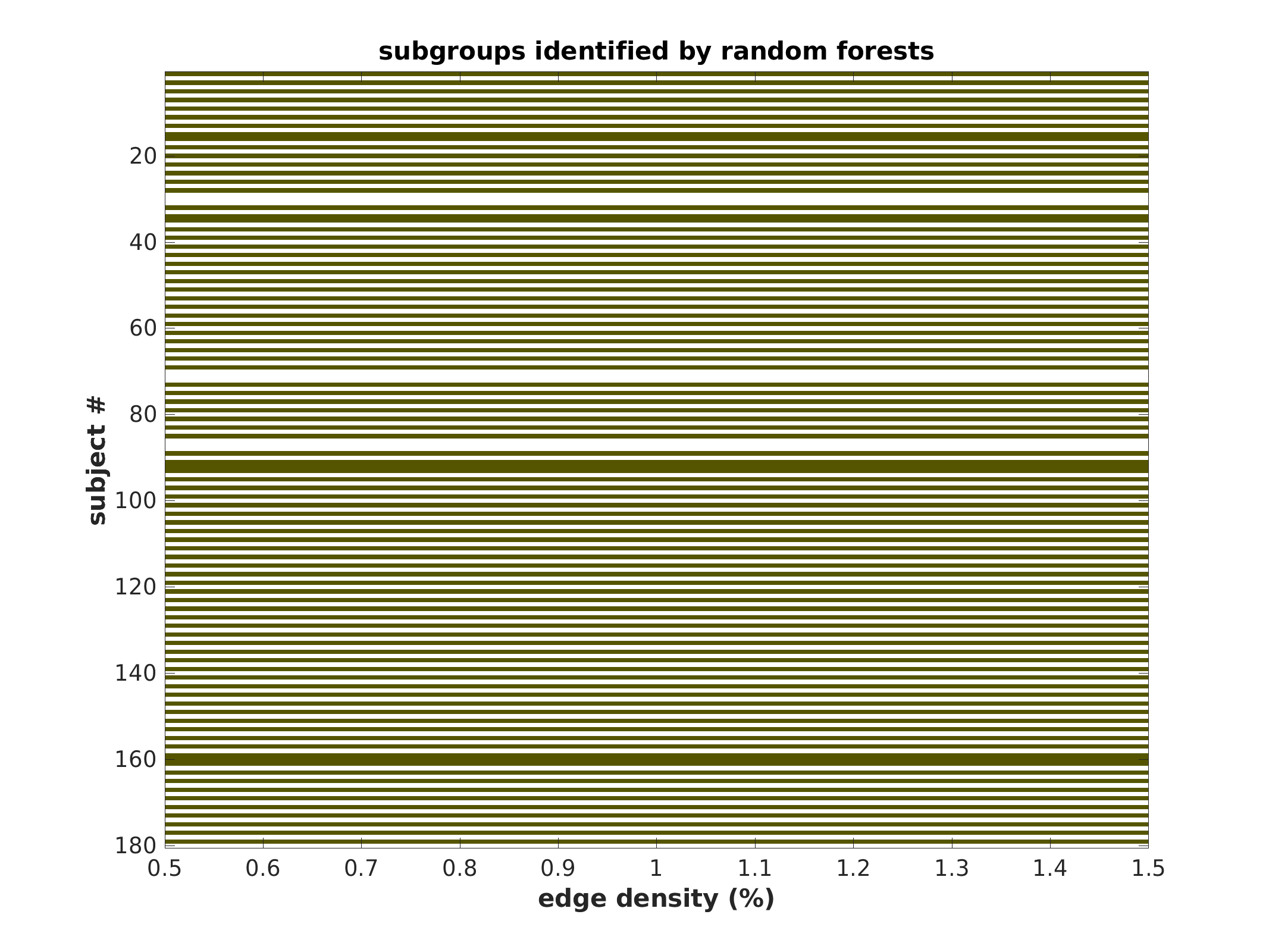
Subgroup community plot (unsorted)
each colored line represents a subject belonging to that color’s subgroup, in provided order
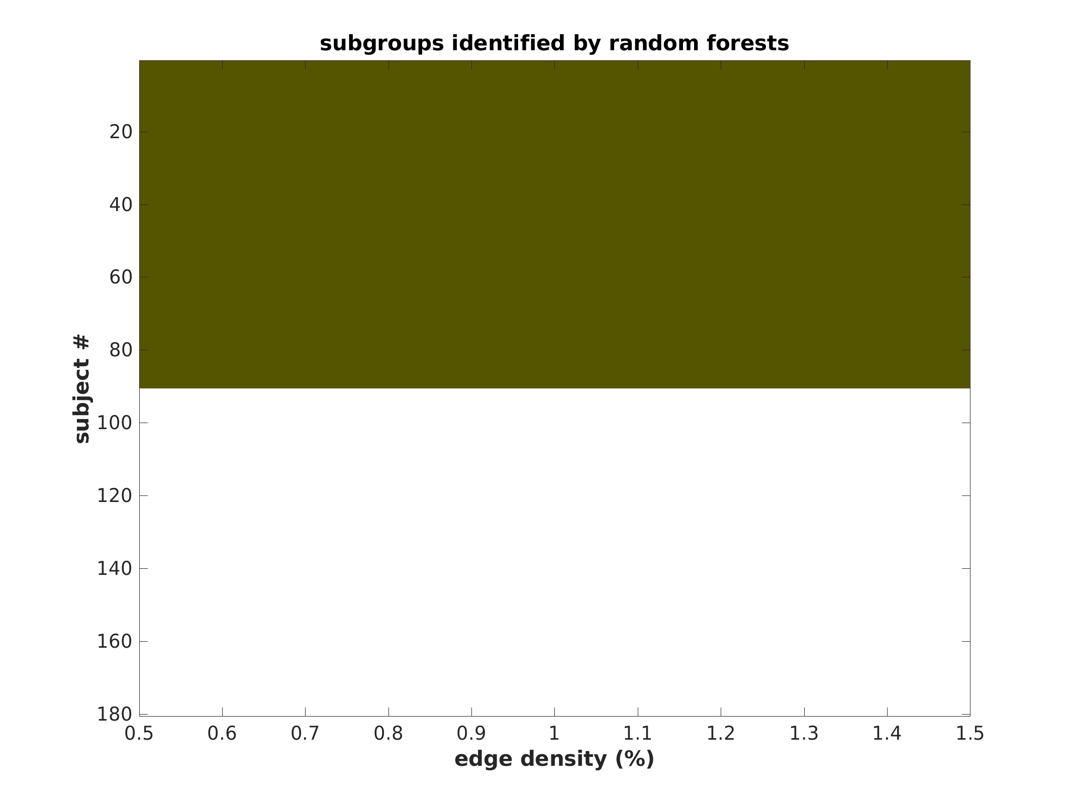
Subgroup community plot (sorted)
same plot as above, except grouped by subgroup to represent population
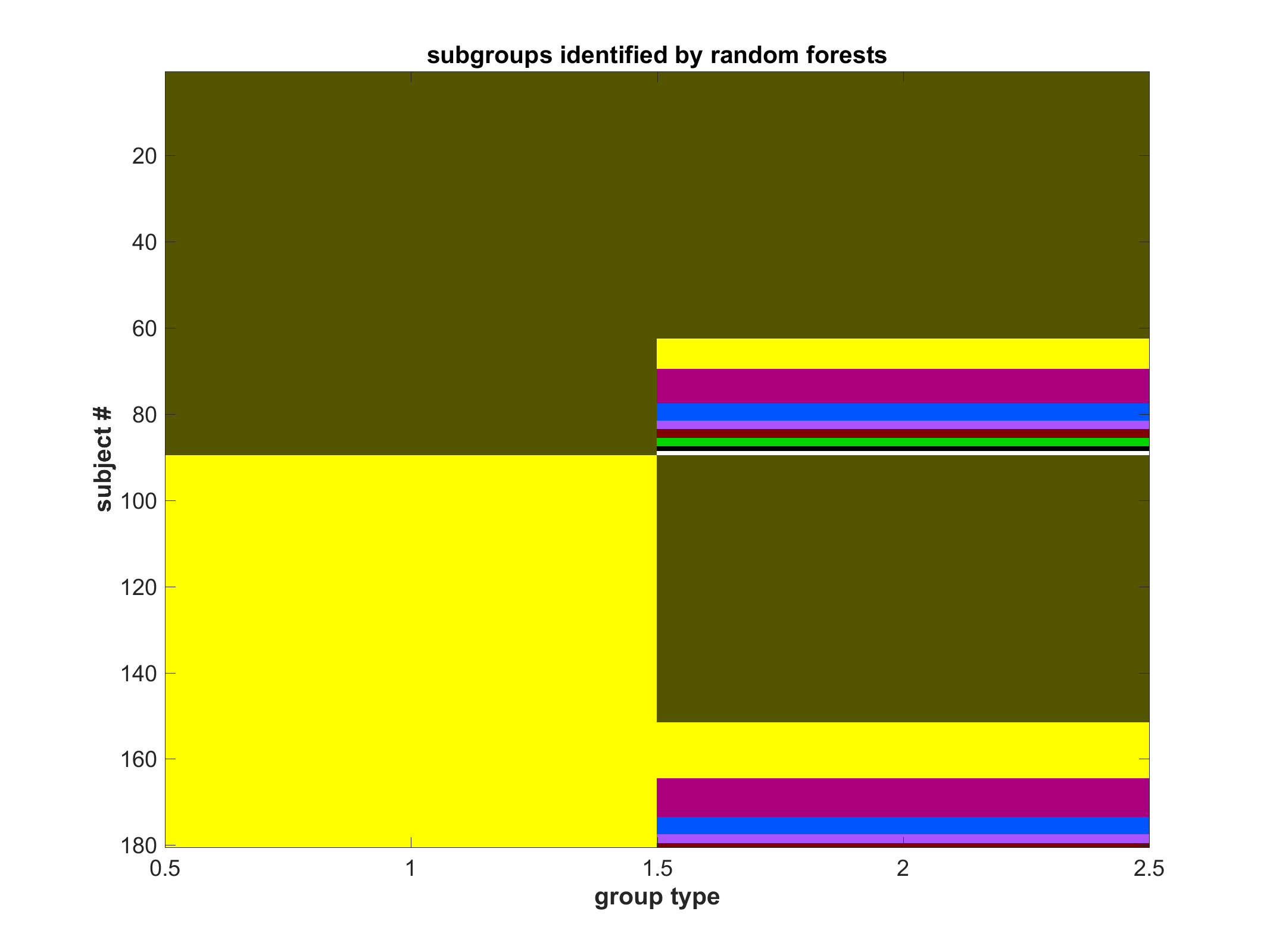
Subgroup community plot with class labels (if available)
Two column plot. Left is classification; Right is subgroup within classification
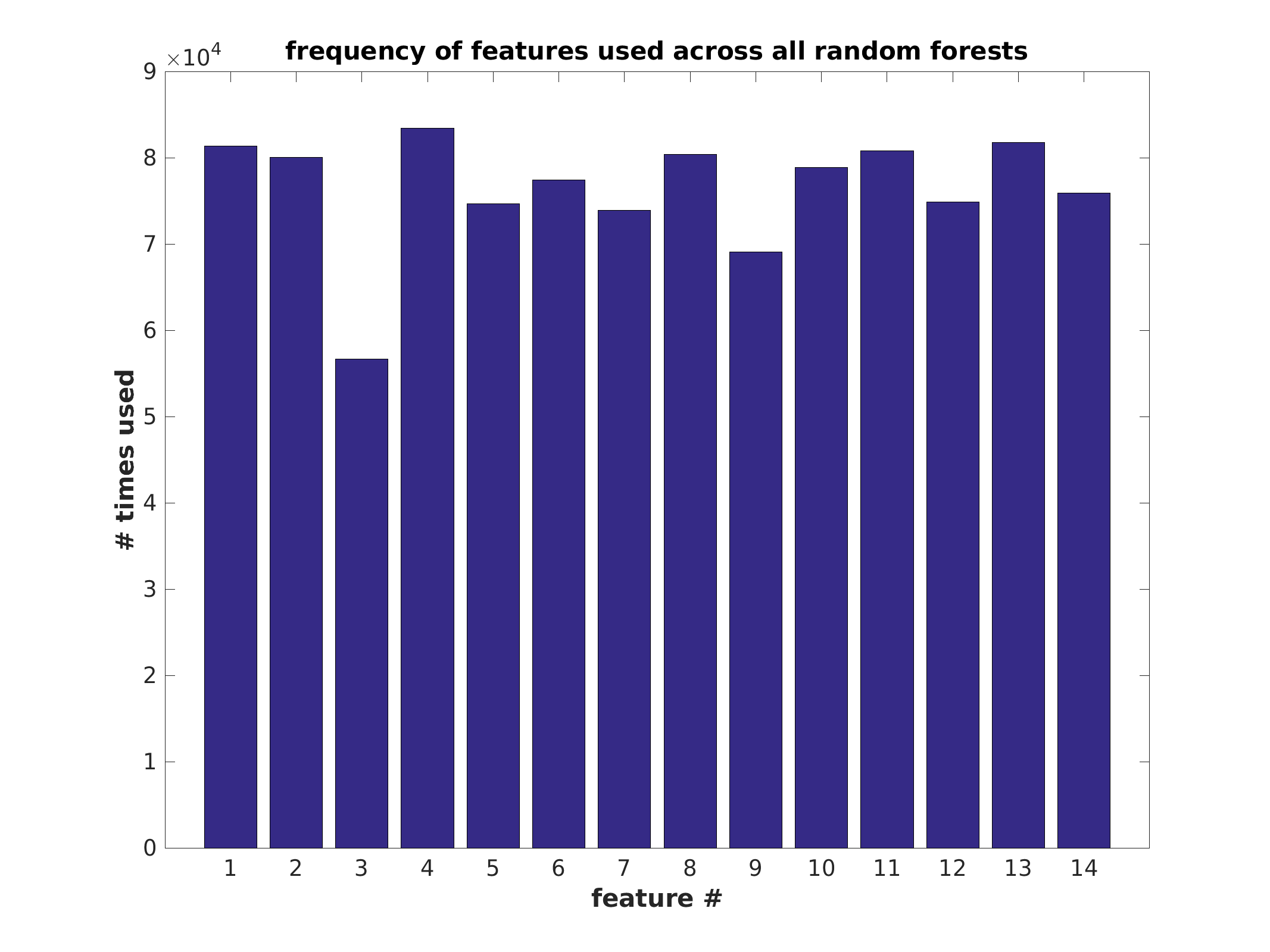
Feature usage
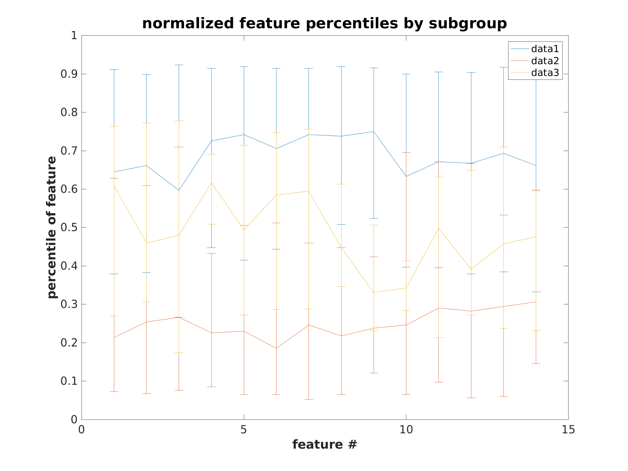
Feature error bar plots by subgroup
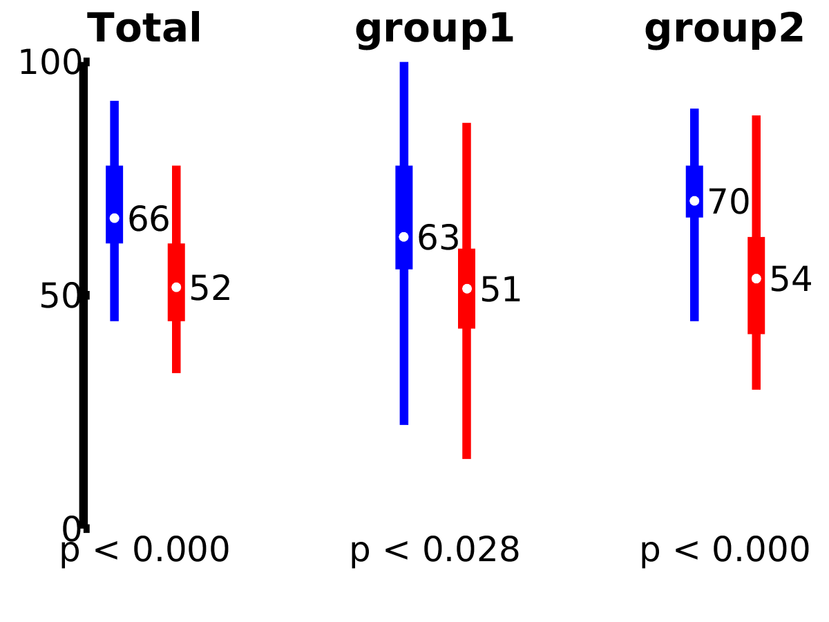
Overall model performance
Guide to determine community detection parameters
Under Construction
Post-hoc strategies for validating subgroups
Under Construction
known bugs and issues
Documentation issues
- Guides for subgroup validation and community detection need to be documented
- Usage of our R scripts needs to be documented
- Data dictionaries for intermediate files need to be documented
- Figure dictionary needs to be generated
- Data visualizations need to be finished
- holdout procedure for twin studies is undocumented
known bugs
- Unsupervised RFSD power analysis may produce inaccurate performance estimates
- Currently, output results are split into a “group1” and “group2” variable even when “use_group2_data” is set to “false”. In this case, “group1” refers to the first half of all rows in the input data, “group2” refers to the second half. This bug remains due to backwards compatability and will be resolved in the next release.
planned features
- enable hyperparameter tuning for RFs, currently, one needs to rerun the FRF to tune hyperparameters
- test and refine holdout code for twin studies